Why We Needed a Carbon Land Standard, and What’s Next Now That We Have One

In the past four decades, we have built up sophisticated machinery for making global climate progress (e.g. we have IPCC, GHGP, CDP, SBTi), but there are two key problems:

1. Our carbon accounting system has not sufficiently accounted for land use emissions—resulting in misaligned incentives in land sector sustainability efforts
2. We don’t have a global compliance mechanism that ensures we achieve our targets 

On January 30, 2026, GHGP published its first Carbon Land Standard, taking a major stride toward fixing how we account for the interconnected carbon cycles of the world's farms and forests.

We’ll be posting a short series of articles that dive into these themes. Here, we’re covering this new standard... and we’ll save the trivial matter of global compliance for another day.

Why We Needed a Carbon Land Standard, and What’s Next Now That We Have One

If we had this framework 30 years ago, we would never have justified clearing a single acre of rainforest to produce ‘low carbon fuels.'

Takeaways:

• GHGP released a new standard that now requires reporting for land-use change emissions and land occupation[1]
• More than half of agricultural emissions stem from land-use change[2], so this new standard closes a critical reporting gap 
• The land occupation requirement marks a first step towards a carbon balance sheet reporting standard—adding a missing dimension for businesses to holistically assess their climate impact
• The standard requires a carbon opportunity cost (COC) analysis for high-leakage businesses—a framework designed to keep climate-motivated land-use decisions from backfiring

The GHG Protocol (GHGP) sets the de facto standard for greenhouse gas accounting, with over 90% of S&P 500 companies disclosing their emissions and following GHGP accounting and reporting guidelines. 

On January 30, 2026, GHGP published its first Land Sector and Removals Standard¹. The new standard requires that GHGP compliant reporting:

• Account for all GHG emissions associated with land-use change (scope 1, 2, 3)
• Account for all land occupation (scope 1, 2, 3)

Let’s take a look at how the measured footprint of common oil crops and fats changes when we implement these requirements. The chart below shows the combined impact of production emissions (taupe) and direct land-use change emissions (dLUC, light green)[3]. This direct emissions footprint is shown alongside carbon opportunity cost (COC, dark green) and land use (gold)[4]. We dig into the weeds below, but with even a cursory glance, we can already highlight a key takeaway:

• Land use almost always dominates the GHG footprint of these crops: so ignoring land's GHG contribution misses most of the impact

Missing this point is catastrophic and has resulted in some of the most perverse outcomes from well-intentioned climate policies. The biofuels industry is a textbook case, where low-carbon fuel programs in North America and Europe incentivized direct and indirect land-clearing of over 1 million hectares of old-growth forest in the tropics for biofuel production[5,6,7]. It will take decades (in some cases centuries) to recover from the carbon debt of this land-use change[8,9]—not to mention habitat and species loss.

It has been both clear and urgent for more than a decade that our GHGP reporting standards need to account for land-use. But it’s taken until 2026 to get here because the accounting methodology has had to contend with a much higher level of complexity and uncertainty than production emissions. Stare at the chart above for a minute, and you may start to see some of the nuance: why are LUC emissions shown on both a ‘dLUC’ and ‘COC’ basis? Why are dLUC emissions shown regionally, but not COC? What drives the relationship between land intensity and COC? 

Before getting into those details, I want to highlight a critical decision GHGP made with this LSR standard that underpins some of those questions:

• by requiring land occupation reporting, GHGP is extending their footprint methodology beyond carbon equivalent fluxes to now include an accounting of carbon stores.

Previous standards have focused entirely on flux accounting: how many net molecules with radiative forcing potential did your company cause to be released into the atmosphere this year? In financial terms, this maps to GHG income statement reporting. The new standard essentially mandates that projects that occupy land must now also report a balance sheet.

And don’t be lulled by the accounting jargon, because this decision is enormous. As it is ultimately the stores, the concentration of IR-resonant molecules in the atmosphere, that drive global climatic shifts, not just the flux from a given year. Extending GHG accountability beyond our annual budgets to what’s actually in our bank account – that is progress.

So how do we turn progress into impact?

GHGP creates the accounting frameworks and reporting standards that corporations follow when reporting their GHG footprint. The measurements and documentation that result from reporting can drive awareness… and sometimes behavior change. But the real lever of change comes from setting and driving towards systematically defined targets that align with our global objectives for climate stability and ecosystem integrity. 

And that’s where SBTi comes in: the Science Based Targets Initiative (SBTi) provides guidelines for corporations on how to set GHG reduction targets. Just as we encountered in creating a land sector accounting methodology, target setting in this sector is not straightforward. 

Most of our global land occupation is for food production. We can’t set targets to reduce land occupation and use without consideration of global population and dietary needs[10]. So setting smart targets will have to hinge on yield improvements and native land disposition—the more food we can produce per land area, and the less natively rich the ecosystems are where we produce foods, the lower the footprint. These two objectives are often opposing, where lands with natively rich ecosystems tend to produce the highest agricultural yields. Carbon Opportunity Cost (COC) accounting, which GHGP introduces in the new LSR Standard, provides a powerful framework for this multifactor optimization. 

Note that in the new LSR Standard, GHGP requires land occupation reporting, while indicating that this reporting may be done on a COC basis, but COC reporting is not a formal requirement in the standard[1]. We expect that the most streamlined target-setting approaches will make use of COC. If we had adopted this framework 30 years ago, we could never have justified cutting down a single hectare of rainforest to produce ‘low carbon fuels’. So, let’s save every hectare that’s left and set credible and achievable targets to start restoring what’s been lost.

Happy accounting!

I’m Just Here for the Methods

Here are the key metrics that we’ll need for implementing the LSR Standard to analyze regional and crop specific drivers of agriculture’s climate footprint.

E_prod = (Σ e_i) × A

E_prod : production emissions. Where e_i is per-hectare emissions intensity, i indexes scope 1, 2, and 3 emissions sources^[1] (fertilizer, energy, transport, processing, etc.), A is land area.

E_dLUC = ((c_before − c_after) / t_amort) × A

E_dLUC : direct land-use change emissions. Where c is per-hectare carbon density (above- and below-ground biomass)^[2][11], A is land area, and t_amort = 20 years per the LSR Standard[1,12]. Booked as a one-time capital ‘expense’, amortized straight-line.

COC = ((c_native − c_actual) / t_amort) × A

COC: carbon opportunity cost. Where c_native is the per-hectare carbon density under the land’s native ecosystem potential^[3][11,13], c_actual is what is currently stored under agricultural use, A is land area and t_amort = 20 years. Booked as an annual liability rather than a one-time expense.

Production Emissions 

Production emissions follow standard flux accounting methods for scope 1, 2 and 3 emissions, such as: emissions from fertilizer production, N2O release, raw material production and transport, downstream processing emissions, energy emissions. In the chart we presented previously (reprinted in the discussion below with some additional data points) you may have noted that the production emissions we used for our dLUC vs COC scenarios have slight differences. In practice, production emissions are measured and aggregated from the farm-level all along the supply chain and are specific to a particular product. But we wanted to show a regional dLUC vs global COC analysis, and so we sourced self-consistent production emissions for each of those cases. 

Direct Land Use Change (dLUC)

The dLUC footprint is calculated by taking the difference between the carbon contained in all the above and below ground biomass before and after the land was converted to agriculture and amortizing the carbon flux over a period. In accounting terms, this carbon transaction is booked as a capital purchase (carbon released upon land conversion) that occurs once and is amortized (straight-line) over 20 years. 

The result is that conversion of a primary forest or peatland to agricultural use will have much higher land use emissions than conversion of degraded agricultural lands in the same region. This favors agricultural expansion into degraded rather than pristine lands (good!), but it doesn’t valorize the opportunity of restoring those degraded lands to native forests (problematic!). After the one-time land conversion expense has fully amortized, the land-use disappears from the books entirely.

The following graph from our Food without Agriculture paper[2] illustrates this very effectively. The land-use emissions of Brazilian soy are 3-6x higher than European or US soy due to a combination of temporal and productivity factors:

• North American and European land conversions happened more than 20 years ago, so is fully amortized
• Brazilian ecosystems are inherently more productive than others[2]

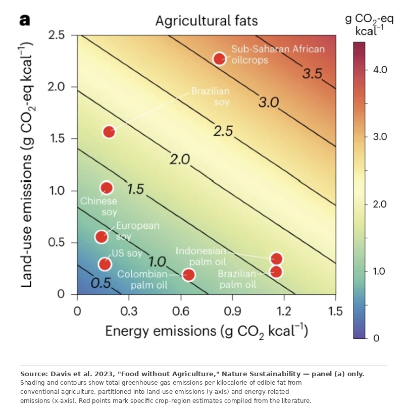
COC provides a more robust methodology for de-coupling this picture to assess and optimize agricultural land transition^[4].

Carbon Opportunity Cost (COC)

Instead of treating the carbon release upon land conversion as a capital transaction that occurs once and is amortized over 20 years, COC analysis characterizes land use more like a lease liability. The difference between the potential stored carbon of a native ecosystem and the actual stored carbon under agricultural use is the foregone carbon opportunity of the land-use. An annual COC is then calculated by dividing the total land carbon opportunity over a similar timeframe as dLUC amortization (ranges between 15-45 years are used in the literature for the amortization period). This cost is booked as an ongoing liability, rather than amortization of a capital purchase.

As a reminder, the LSR Standard requires COC for quantifying land carbon leakage for activities at high-risk of leakage, but it does not require COC for general land occupation reporting—if a business does is not considered high-leakage risk, then occupation can be reported as total hectares occupied. However, land occupation misses the important dimension of land productivity that is captured in a COC analysis. 

For example, consider oilpalm grown in South East Asia (SEA)—the world’s highest-yielding crop on a caloric basis. If you are reporting and setting targets related to total land occupation rather than COC, you may easily converge on a strategy that minimizes your total land occupation by maximizing your use or development of oilpalm in SEA. However, once you factor in the native productivity of the lands—the carbon opportunity cost—we find better alternatives that bias towards preservation of SEA ecosystems. 

Because of cases like this, we’d argue that COC is a more sophisticated assessment tool for incentive-aligned decision making than land-use alone, and should be a default in the SBTi guidelines.

Discussion & Further Analysis

Putting all these concepts together brings us back to the chart we started with (a few additional crops included for this discussion). We now have the tools to understand the differences between dLUC and COC, with COC representing the total carbon storage opportunity of a land area that is foregone due to agricultural production, and dLUC being the explicit emissions footprint of a given crop, both mapped onto an annual basis. Additionally, the relationship between land use and COC can now be interpreted, with COC functioning as a composite metric, accounting for both native land productivity and land intensity. 

There are times when COC and dLUC will converge to similar values, but they are fundamentally different constructs that tell us different things. To summarize:

• Reference Carbon Stores
• dLUC: compares current land use with most-recent disposition prior to current agricultural conversion
• COC: compares current land use with native land potential, can be calculated as either
• global analysis: weighted average native land potential across all global regions where a crop is grown
• regional: native land potential across a specific region of interest
• Mechanism
• dLUC: net released carbon due to land conversion, amortized over 20 years
• COC: land carbon opportunity, annual liability with 20 year basis 
• Termination
• dLUC: no contribution after initial LUC is fully amortized
• COC: annual liability tied to land occupation that does not terminate
• Restoration
• dLUC: reversed if land is restored to its original state; negative if land is restored to a richer ecosystem state than baseline
• COC: approaches zero as land restoration approaches native ecosystem state

Going a level deeper on our fats and oils example, let’s revisit the regional and crop variations for soy and palm from our 2023 paper[2] to compare the dLUC and COC frameworks. In the following chart, the dLUC data points correspond to the data points called out on the land-use emissions vs energy emissions colormap above, and we’ve charted them alongside a COC analysis on both a regional and global basis. 

A few key takeaways from this chart.

COC is usually higher than dLUC. This is because it doesn’t come off the books when land conversion emissions have been fully amortized, and it always references native ecosystems, not just the most recent state of the land prior to its current disposition.

Brazilian soy (Cerrado) is a notable exception, with dLUC (17.8) > COC (10.1). This reflects active clearing in the carbon-dense Cerrado frontier (and some lingering Amazon conversion in the 20-year amortization window), while COC averages regrowth potential in each specific biome—with Brazil’s Amazon COC being more than 2x higher than Brazil’s Cerrado COC.

dLUC and COC tell two different stories. dLUC is high where deforestation is currently amortizing and low where the clearing happened decades ago — useful, since it indicates whether a specific supply chain is tied to active or recent deforestation. COC reflects the full opportunity cost relative to the underlying ecosystem, independent of historical context – useful for system-level carbon opportunity optimization.

Which framework should you use? This answer is, of course: both. dLUC analysis drives companies to source from regions that have not had recent land-clearing, which discourages contributing to new deforestation. But it fails to incentivize progress like optimizing a crop for higher yields on fully amortized agricultural lands, while COC captures the ongoing carbon impact of land-use. 

However, within COC analysis, there is another layer of nuance. You’ll note that we have included both regional and global COC analyses in the chart above. If a company is analyzing their COC, which approach is more relevant? Here, I would say: it depends. Regional COC analysis is helpful for understanding the regional carbon potential of different lands, so it is useful in evaluating agricultural land transition (either expansion or contraction). However, global COC is the value that belongs on the balance sheet—which is why we report global COC as default and have only shown a regional COC analysis in this final deeper dive chart. The reason for this comes back to leakage: if you switch your soy supplier from Mato Grosso to Iowa, you haven’t reduced global emissions. Another buyer will take your place in Brazil. Keeping global COC on the balance sheet drives crop-level accountability and is needed to inform longer-term strategy like improving yields and transitioning to less ecosystem-intensive crops. 

Reporting both dLUC and COC is like reviewing both an income statement and a balance sheet. There's a reason this is standard in financial reporting: you want to know whether you're cash-flow positive year over year, and you want to know your overall financial position. By getting both of these metrics into the GHG reporting standard, GHGP has dramatically improved the assessment framework for setting land-sector targets. SBTi guidance for the land sector should follow suit.

Supplemental Note 

There is a whole other part of the standard that I haven’t addressed at all; it is about removals. It is beyond the scope of the present discussion, but is an incredibly important part of the framework for two reasons:

• It creates a mechanism to incentivize carbon removals: where the credit for increasing the stored carbon in geologic features or natural ecosystems can be annually credited to a company engaging in and monitoring sequestration and ecosystem restoration.
• It opens the door to a much-needed balance sheet accounting mechanism for non-land-sector industries. 

(It appears that someone has made a quite thoughtful effort to combine these land and removals components in the same Standard; I’m honestly impressed.)

References

1. GHG Protocol, "Land Sector and Removals Standard," v1.0 (January 2026). https://ghgprotocol.org/sites/default/files/2026-01/Land-Sector-and-Removals-Standard.pdf

2. K.A. Davis, K. Alexander, et al., "Food without agriculture," Nat. Sustain. 7, 90–95 (2024). doi: 10.1038/s41893-023-01241-2 https://www.nature.com/articles/s41893-023-01241-2

3. C. Hong, J.A. Burney, J. Pongratz, J.E.M.S. Nabel, N.D. Mueller, R.B. Jackson, S.J. Davis, "Global and regional drivers of land-use emissions in 1961–2017," Nature 589, 554–561 (2021). doi: 10.1038/s41586-020-03138-y https://www.nature.com/articles/s41586-020-03138-y

4. World Resources Institute, Cool Food Calculator. https://www.wri.org/initiatives/cool-food

5. Trase / Stockholm Environment Institute, "Indonesian palm oil exports and deforestation" (2024). https://trase.earth/insights/indonesian-palm-oil-exports-and-deforestation

6. K.G. Austin et al., "Shifting patterns of oil palm driven deforestation in Indonesia," Land Use Policy 69, 41–48 (2017). doi: 10.1016/j.landusepol.2017.08.036 https://www.sciencedirect.com/science/article/pii/S0264837717301552

7. T. Searchinger, R. Heimlich, R.A. Houghton, F. Dong, A. Elobeid, J. Fabiosa, S. Tokgoz, D. Hayes, T.-H. Yu, "Use of U.S. croplands for biofuels increases greenhouse gases through emissions from land-use change," Science 319, 1238–1240 (2008). doi: 10.1126/science.1151861 https://www.science.org/doi/10.1126/science.1151861

8. J. Fargione, J. Hill, D. Tilman, S. Polasky, P. Hawthorne, "Land Clearing and the Biofuel Carbon Debt," Science 319, 1235–1238 (2008). doi: 10.1126/science.1152747 https://www.science.org/doi/10.1126/science.1152747

9. H.K. Gibbs et al., "Carbon payback times for crop-based biofuel expansion in the tropics: the effects of changing yield and technology," Environ. Res. Lett. 3, 034001 (2008). doi: 10.1088/1748-9326/3/3/034001 https://iopscience.iop.org/article/10.1088/1748-9326/3/3/034001

10. T. Searchinger, R. Waite, C. Hanson, J. Ranganathan, "Creating a Sustainable Food Future: A Menu of Solutions to Feed Nearly 10 Billion People by 2050," World Resources Report (World Resources Institute, 2019). https://www.wri.org/research/creating-sustainable-food-future

11. S.A. Spawn, C.C. Sullivan, T.J. Lark, H.K. Gibbs, "Harmonized global maps of above and belowground biomass carbon density in the year 2010," Sci. Data 7, 112 (2020). doi: 10.1038/s41597-020-0444-4 https://www.nature.com/articles/s41597-020-0444-4

12. IPCC, 2019. 2019 Refinement to the 2006 IPCC Guidelines for National Greenhouse Gas Inventories, Volume 4 (Agriculture, Forestry and Other Land Use). https://www.ipcc-nggip.iges.or.jp/public/2019rf/index.html

13. S.C. Cook-Patton et al., "Mapping carbon accumulation potential from global natural forest regrowth," Nature 585, 545–550 (2020). doi: 10.1038/s41586-020-2686-x https://www.nature.com/articles/s41586-020-2686-x